Linear regression for assessing and predicting the market value of used cars
1. Introduction
The purpose of this blog post is to explore the possibility of applying linear regression to describe, analyze and predict the listing price of used cars. In this regard, linear regression is introduced more loosely without having to define concepts in a strict mathematical sense. The data used in this post is scrapped from major used car listing websites. For more on the data and the subsequent analysis see this Jupyter Notebook or see the ‘Data’ section below. A serverless API of the final model is available here. You can also checkout my Github page if you are interested in the python code used for scrapping or if you want to download the data in csv format.
To make like-for-like comparisons and analysis, the following mid-sized sedans are considered.
| Manufacturer | Model |
|---|---|
| Toyota | Camry |
| Honda | Accord |
| Nissan | Altima |
| Ford | Fusion |
| Hyundai | Sonata |
| Chevrolet | Malibu |
| Volkswagen | Passat |
The goal is to be able to address questions like:
- How much would a model X car that is driven Y miles cost?
- What is the average price of model X cars after Y miles of usage?
- How much does depriciation (w.r.t. mileage, release year) affect model A cars compared to model B?
That said, everything stated in this blog post is solely based on curiosity and the desire to apply regression to the used car market. Obviously, anyone seriously considering to buy a car should seek expert advice.
2. The theory
Linear regression inherently assumes that there is a linear relationship between a random variable (the dependent variable) and another set of random variable(s) (the independent variables), i.e,
,
where is called the intercept and is the coefficient for . Often, the independent variable and the coefficients are expressed as -dimensional vectors, i.e., and
Linear regression acknowledges the relationship between the dependent and independent random variables can be non-deterministic. That is, there can be some uncertainity involved in determining the value of Y evenif we have a perfect knowledge of the values of the s. This uncertainity is represented by the error term e in the regression equation. All the uncertainity we cannot (or don’t want to) explain about Y is absorbed by this term.
In order to build reliable models we make the following assumptions on the error term:
-
The error should be independent of . For example, let our linear regression model represent the power consumption of an electronic device as a function of the load, and let us assume the model is ( and representing the and random variables, respectively). The independence assumption dictates that the probabilistic nature of should remain unaffected whether the load is 10%, 95%, or any other value.
-
The spread of e remains constant across all values of X. Going back to the previous example, e should not be more (or less) spread for the range of load values under study.
-
If statistical tests are required, we further need to assume that e has a normal distribution centered at 0. For further details on related matter check the assumptions and best practices of linear regression.
The coefficients in a linear regression model can be solved directly by matrix inversion or more iteratively by gradient descent or one of its variants.
Here it is important to note that the ‘linear’ in linear regression does not necessarily mean the relationship between X and Y is expressed as a straight line. For example,
is also considered a linear model as long as the expression remains linear in the coefficients.
Clearly, there is a plethora of models to choose from. we, therefore, need to have metrics that quantify how well a model performs in capturing the relationship between X & Y to be able to select the best model. Two of such metrics are:
-
R2: Also refered to as the coefficient of determination indicates how much of the variability of Y is explained by X (the independent variable). R2 of 1 tells us X perfectly (100%) explains the variability in Y, i.e., there is no uncertainty left in Y once the values of X are known. By contrast, R2 of 0 suggests X does not explain any of the variability in Y at all. Other values between 0 and 1 lie on the spectrum accordingly.
-
Predicted R2 and Adjusted R2: One weakness of R2 is that it is susiptible to overfitting. Predicted R2 and Adjusted R2 are aimed at mitigating this issue. Read this post for more detail.
-
RMSE: The Root Mean Squared Error is the expected magnitude of prediction error. RMSE = 0 represents a perfect model, and model performance decreases as RMSE increases. RMSE can also be nicely decomposed into bias and variance terms of the model.
We will also apply confidence and prediction intervals. This video elegantly shows what their difference is and how to calculate them.
3. The data
The data, as already mentioned in the introduction, is scrapped from car listing websites. The scrapped data is parsed and cleaned and the resulting data is stored in a csv file, which has the following format:
| Year | Year of release, e.g. 2010, 2019 |
|---|---|
| Make | Manufacturer of the car: Honda, Toyota, Nissan, Ford, Hyundai, Chevrolet and Volkswagen |
| Model | Accord, Camry, Altima, Fusion, Sonata, Malibu or Passat |
| Model detail | Trim level, e.g. for Honda LX, Sport, EX, EX-L and Touring |
| Price | Listing price of the car |
| Mileage | Mileage (in miles) posted by dealer |
| Website | A two letter abbreviation to identify the source website |
The following table provides valuable summary statistics of the quantitative columns
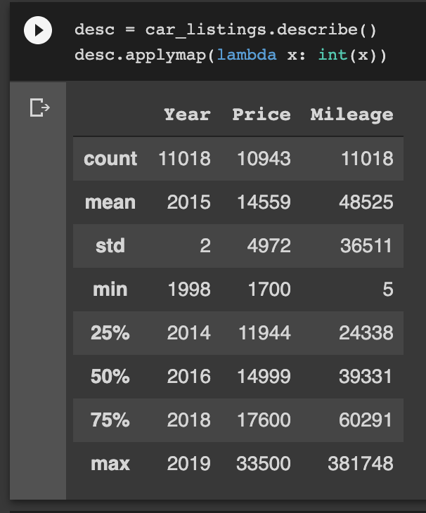
The CSV file contains listing details of 11,018 cars. However, dealers may list the same car more than once to improve its chance of being discovered among other cars. Duplicate entries may lead to inaccurate analysis and prediction. We, therefore, need to remove duplicates and run the summary statistics again. Doing so reveals that about half of the listings are duplicate entries as shown below.
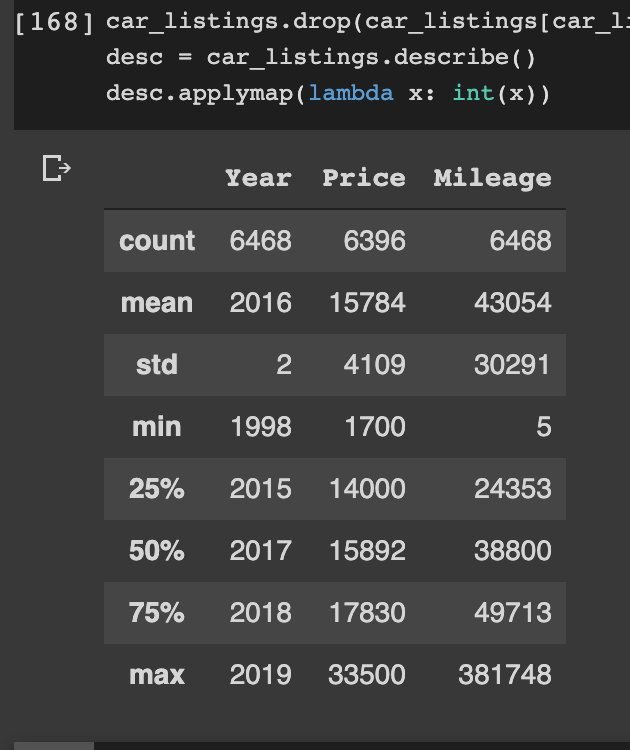
Now we know that there are 6396 unique cars. Going one level deeper, we can see the number of cars, the average price, average mileage and average release year per manufacturer (model) below
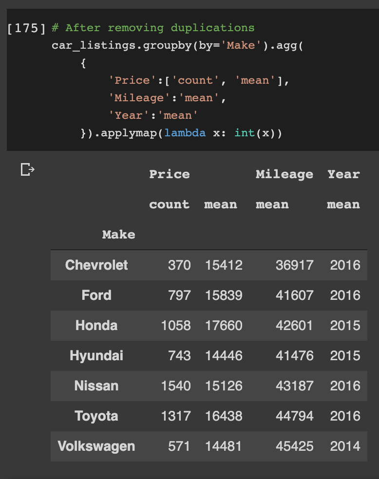
Out of the 6396 unique cars listed, 1540 are Nissan Altima, 1317 are Toyota Camry, 1058 are Honda Accord and so on.
4. Analysis
Here, the goal is to build a multi-linear regression model that predicts (summarizes) the Listing Price of a used mid-size sedan car based on its Mileage, Release (Model) Year, and Trim level. We’ll build separate regression models for each of the cars listed above, excluding VW Passat and Chevrolet Malibu.
Before jumping into building the regression models, let us examine how Price tends to change with respect to Mileage and Year by taking the Honda Accord data set as an example. The following plots reveal the strong negative relationship between mileage and price and the strong positive relationship between release year and price.
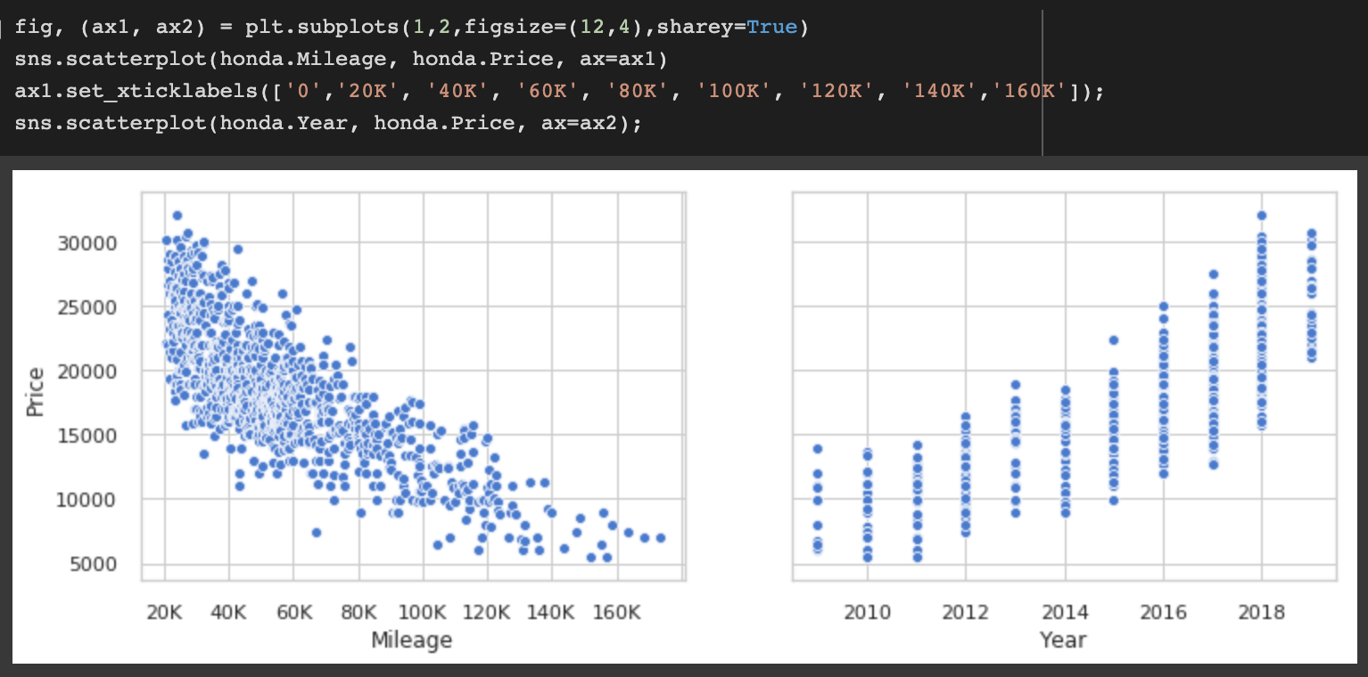
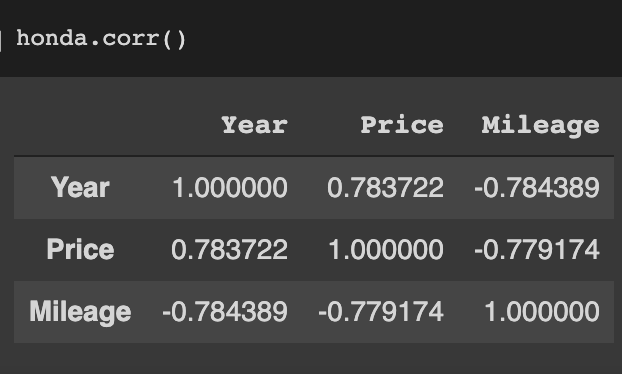
The correlation matrix shown below quantifies this relationship. It also shows the strong negative relationship between Mileage and Year. Intuitively, it is highly unlikely for a 2019 model to rack up 100,000 miles as it is equally unlikely for a 2008 model to have a mileage of 10,000 miles.
For more on this and other analysis related to regression model building see this python notebook.
4.1 Regression models
After considering a number of features and feature transforms the following regression function that better expresses the relationship between the independent variables (Mileage, Year, Trim level)and dependent variable (Listing Price)is chosen:
,
where are the Price, Mileage, Year, and Trim of car , respectively. are the intercept, coefficient w.r.t Mileage, and coefficient w.r.t. Year. Since trim level is a categorical variable, we need to dummy-encode it before it can be used in a regression model. Assuming there are trim levels of a car model dummy variables are created using the summation of the indicators in the last term of the above equation. This results in one dummy variable for each trim level except the base trim-level. Coefficeint , therefore, represents the price difference between the base trim level and the trim level.
Note that Mileage and Year are transformed using functions and . The log transformation of Mileage not only yields better model performance it can also be motivated by the fact that the sharpest decline in Price happens during the first few (thousand) miles. Once a car makes it into tens of thousands of miles, the rate at which the Price decreases should slow down. Logarithmic functions are one of several functions that could capture this nonlinear relationship between Mileage and Price. Since base 2 logarithm is used, $a_1$ represents the depreciation with respect to mileage every time mileage doubles.
When it comes to the Year, what affects the Price of a car is how old the model is relative to the newest model, which is why the transformation is used. For example, a Toyota Camry is years old and should have a lower price than a ( years old) Toyota Camry if everything else is kept constant.
Five elastic net regularised models are trained for Ford Fusion, Honda Accord, Hyundai Sonata, Nissan Altima, and Toyota Camry. The coefficients and performance metrics of the resulting models are shown below.
| Car Model | Count* | Coefficients() | * | RMSE($) |
|---|---|---|---|---|
| Ford Fusion | 743 | (-1180, -920) | 81.2% | 1543 |
| Honda Accord | 1015 | (-1350, -1050) | 87.2% | 1888 |
| Hyundai Sonata | 687 | (-1200, -770) | 80.3% | 1302 |
| Nissan Altima | 1434 | (-1250, -780) | 70.9% | 1217 |
| Toyota Camry | 1172 | (-770, -1010) | 77.2% | 1510 |
- score is calculated on a test set after outlier removal using Cook’s distance. The number of cars used to train each model after outlier removal is presented in the ‘Count’ column.
According to the regression models, Toyota Camry has the smallest (in magnitude) coefficient w.r.t Mileage at . Take, for example, the price of a given Toyota Camry is at 500 miles. The model predicts that the average price drop is $19,230$ at 1000 miles, $18,460 at 2000 miles, so on.
Note that coefficient represents the depreciation with respect to mileage, which makes Toyota Camry the best one among the five models considered for retaining much of its original value as mileage increases. By contrast, Nissan Altima and Hyundai Sonata exhibit the least depreciation with respect to Year, with every passing year reducing the value of the car by about $800.
The following plots show the fitted regression models for all car models along with the data used to fit the regression models. In order to simplify the plots into 2D, cars (points in the scatter plot) are assumed to rack up 12000 miles per year, allowing us to represent Year in terms of Mileage as .
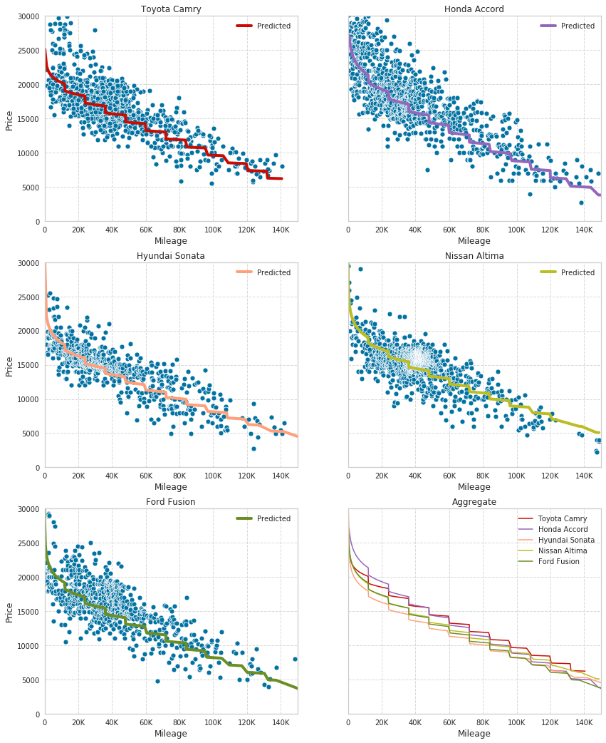
The bottom right plot shows all five regression curves in one plot. This plot, once more, gives the visual confirmation that Toyota Camry loses the least amount of value to depreciation.
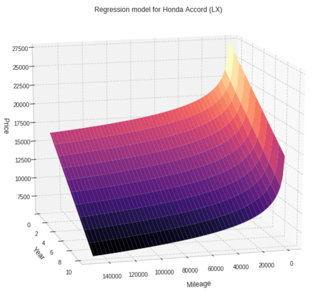
Without the 12000 miles/year assumption, the resulting plots are 3-dimensional. The next figure shows such a plot for Honda Accord. It is easy to see that Price decreases linearly in the Year axis and logarithmically in the Mileage axis.
4.2 Prediction and comparison
The regression models we built can be used to predict the value of a car as well as making inference. Typcial questions we are interested in prediction are “What is the average price of used cars from model X, Year Y, trim T with mileage M?” or “What is the price range for a particular used car from model X, Year Y, trim T with mileage M?”. The former question is answered using the the regression line and calculating a confidence interval around it, while the latter is addressed by calculating a prediction interval along the regression line.
For example, the predicted average price of the base trim-level (LE) 2016 Toyota Camry cars at 40000 miles is
with a narrow 95% confidence interval of while the 95% prediction interval is . Roughly speaking, this means there is a 95% chance that a 2016 Toyota Camry LE car will have a listing price between and at miles.
If we compare these numbers to a 2016 Hyundai Sonata car at 40000 miles, we get
with confidence and prediction intervals of and , respectively.
In some cases, the prediction intervals can be too wide to be useful, specially compared to the narrow confidence intervals for the average listing price. However, considering the long list of factors that can affect the price of a car, this should not be surprising since the regression model only uses mileage, year, and trim level to predict price. The intervals could be narrowed down by obtaining more data and including additional features such as engine type, repair history and accident history.
5. Conclusion
This post illustrated how a simple approach such as linear regression can be applied to infere and predict the listing price of used mid-sized sedans. While regression can be a valuable tool to predict a continuous valued dependent variable, it also sets some assumptions about the predicted and predicting variables that need to be checked before the resulting regression model can be deemed acceptable.
Once the assumptions are checked, regression models can easily be trained with a relatively small amount of data, and in addtion to it’s predictive power, the coefficients of the model also give some insight on the magnitude and direction of the relationship between the dependent and independent variables.