Horizontal scaling and cost-performance optimization
In horizontal scaling systems, resources are added (launched) when the demand on the system increases and removed (stopped) when demand drops and they are not needed anymore. The arrival intensity and the size of jobs processed in such systems usually exhibit a great deal of random variation.
Obviously, having as many resources as possible helps in reducing the latency (response time) experienced by jobs. However, this usually comes at the expense of increased operating cost, e.g., rental, energy or other related costs.
The challenge: To optimize the trade-off between system performance and operating cost
in the face of randomly varying traffic/load. To make things a bit more challenging,
there is also the so-called launch (setup) delay, the time it takes to launch/start a
stopped resource. This could especially be problematic during traffic surges, in which
case resources are launched in response to traffic increase but they are not ready yet
to provide service.
System architecture
Horizontal scalability is a basic system design feature that appears in many (seamingly unrelated) domains. To name a few, call center staffing, inventory management and highly-available and fault tolerant cloud computing all leverage the benefits of horizontal scaling, and hence need to address the cost-performance trade-off mentioned above.
In call centers, fewer operators would translate into less cost (salary) but also longer call waiting time for customers. By contrast, increasing the number of operators would reduce call waiting time but also increase the operating cost. The launch delay, in this case, is the time it takes to (interview, …etc) aquire new operators.
Similarly in a cloud computing environment, virtual machines, containers or lambda functions can be launched/stopped to improve/reduce performance/cost. If the group of resources are virtual machines, the launch delay is the time it takes to bootstrap a VM or start a golden image. In any case, a horizontally scaling system has the following basic components:
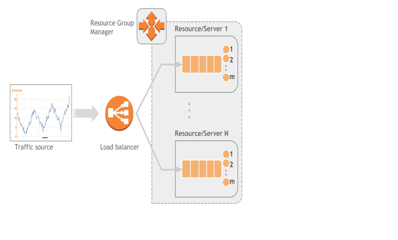
- Traffic source: The stream of jobs that the system is designed to serve. The traffic contributes two sources of randomness that should be considered in the design phase: Inter-arrival times of jobs and their sizes.
- Resource/Server: A server has m service places, in which it can serve m jobs simultaneously. If the number of jobs j is greater than m, the server applies some scheduling policy (e.g. FIFO, PS) to determine which jobs get processed and which jobs wait in (a) queue(s).
- Dispatcher: This is the interface jobs will encounter when they first arrive in the system. Its main duty is assigning incoming jobs to available servers. A dispatcher can be designed to inhance service availability and fault tolerance, in which case it is usually known as a load balancer. A dispatcher may also be designed to unbalance load, e.g. to reduce the cost of running servers by packing jobs to as few servers as possible. The dispatcher employes popular algorithms such as Round Robin, Join the Shortest Queue (JSQ) or Random to assign jobs to servers.
- Resource Group Manager: This manages the cluster of resources/servers. Having a total of N servers at its disposal, of which n<=N are currently active, it applies some scaling policy to determine the number of servers to launch or stop/remove based on current or estimated load.
The following figure shows a black-box representation of each of the components discussed above and their interaction.

Analysis
Quantitative analysis of horizontally scaling systems can be performed using one of the following approaches.
- Measurement and statistical analysis: This is usually the prefered way of analysis, in which relevant data such as request/job arrival times, response times, and the associated cost is collected from an actual system. Statistical analysis of the collected data usually produces valuable insights into the currently implemented system. These insights, however, are limited to the specific system and data set. It is difficult to address questions like “what would happen to the total cost if the request arrival intensity is doubled and the processing power of servers is trippled?” Moreover, such data may not be available, e.g., during the design phase.
- Emulation and detailed model simulation: In this case, a simulator that closely mimicks the internal workings of the system is used to study performance/cost under different scenarios. Once the simulator is built, the system can be studied under all sorts of traffic intensity, load, and cost models. However, this approach requires a fairly detailed model for the analysis to produce a useful result. For example, in the cloud computing system, we may need to model jobs at TCP-connection level or even at packet level (e.g. using NS3).
- Abstract model simulation: Here all interactions are abstracted into stochastic models and each component is treated as a black-box. The traffic is assumed to be generated from a specific random process, whose stochastic properties may or may not be known. Response times are also assumed to be drawn from some (unknown) probability distribution. The black-box approach enables us to quickly develop the simulator and the resulting analysis has a better chance of being generalizable.
- Mathematical analysis: In this case, well-developed mathematical frameworks are applied to analyze the system and quantify performance & cost metrics. Closed-form expressions can be obtained that provide a number of useful insights about the system. However, due to the shear complexity of such systems it often impossible to do mathematical analysis without making some assumptions that may not hold in the real system. Some of the common assumptions are i.i.d. job inter-arrival times, i.i.d service times and stationary (often Poisson) arrival process. The analysis often focuses on mean values of performance and cost metrics instead of percentiles (e.g. 95th, 99th).
Example: Abstract modeling and analysis of a horizontally-scaled AWS-hosted application
As an example of a horizontally scaling system, consider a hypothetical application hosted in a highly available and fault tolerant AWS environment consisting of an Elastic Load Balancer (ELB) and a group of EC2 servers managed in an autoscaling group. Each EC2 instance is configured to run m copies of a specific application. Minimum and maximum number of servers is set for an autoscaling group to limit the extent to which scaling actions can increase/decrease the number of servers. The cost-performance trade-off of this system can be studied by building a simple stochastic simulator. See this mini python package.
AutoScale estimates the load on the system by observing the system for some time. It then takes scale up/down actions based on the estimated load. One way to do that is by setting a target load and a threshold. Servers are launched when the actual load is greater than the target load + threshold, whereas servers are shutdown when the actual load is less than target load - threshold. The threshold helps in avoiding oscillatory effect by the autoscaler while it attempts to keep the actual load exactly equal to the target load by launching/stoping servers indefinately. When a server is marked for stopping, this is communicated with the load balancer so that it stops sending new requests to that server For more on AWS autoscaling please refer the Autoscale user guide.
Elastic Load Balancer (ELB) primarly uses Round Robin (RR) for request forwarding but it can also use least outstanding requests routing (also known as JSQ)in the classic ELB case. For more on ELB please refer the ELB user guide.
In this simulation study the following numerical values are used. The autoscaling group contains a
minimum of 5 and maximum 20 EC2 instances. All instances are on-demand instances.
Each instance runs 8 copies of an application so that
8 requests can be served simultaneously. Requests arrive to the system with an average arrival rate of
40 requests/min and each request on average requires 2 mins of service. Furthermore, inter-arrival times and
service times are assumed to be (exponentially distributed) random variables, but data
collected from real system logs can also be used.
Each EC2 server (in the simulator) could be in one of the following states: stopped, launching, idle or
busy. In the stopped state no cost is incurred. In all the other states cost is incurred at a rate
$0.4/hr, which is roughly the on-demand price of a 2xlarge t3 instances.
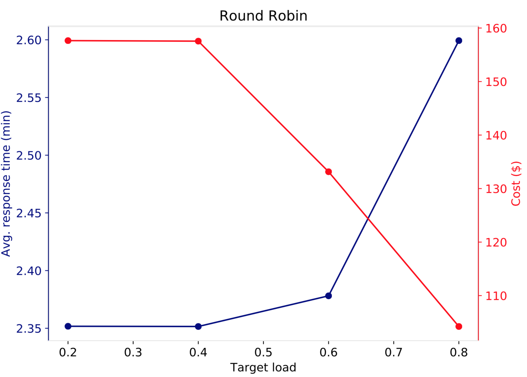
Two sets of simulations are run. In the first set, Round Robin is used at the ELB and target load values 0.2,0.4,0.6 and 0.8 are considered. Note that when the target load is small (e.g. 0.2) more servers are launched than when the target load is large (e.g. 0.8). Thus, application performance should improve when target load decreases while cost increases. The following figure illustrates this.

The right y-axis (red) shows the total cost of the system as a function of the target load (x-axis) after serving 50,000 requests, and the left y-axis shows the average response time of the 50,000 requests. Increasing the target load from 0.2 to 0.4 does not change much both interms of performance and cost. On the other hand, when target load is further increased to 0.6, system cost decreases from around 158 to 132 (about 15% decrease) but average response time increased by less than 2%. Further increasing the target load to 0.8 increases average response time by about 10% and decreases rental cost by an additional 20%.
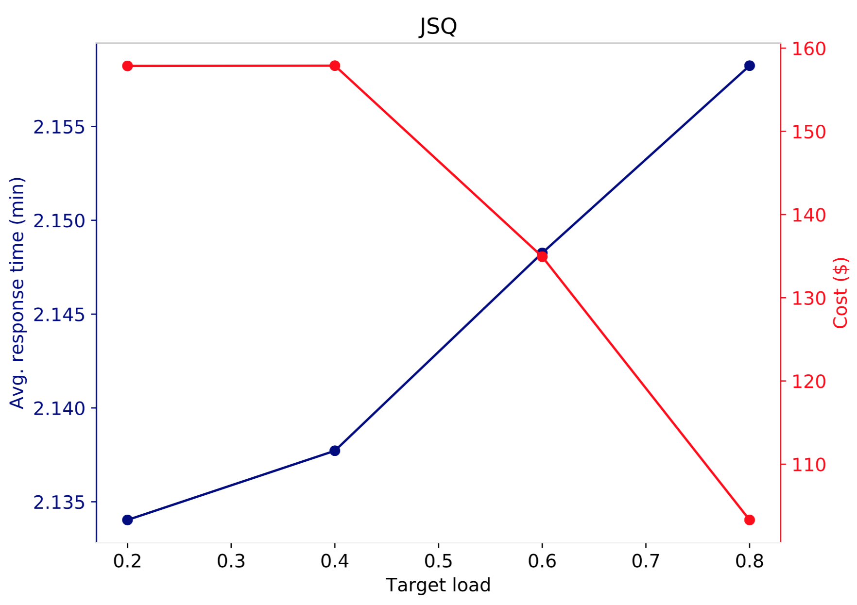
In the figure below, the cost-performance trade-off is shown for the second set of simulations using JSQ as the routing algorithm at the ELB. While the results look qualitatively the same as in the Round Robin case, the average response time curve depicts that JSQ performs better than Round Robin. That is, for the same amount of dollar spent, JSQ gives better performance than Round Robin. This is in fact a well known result, and the advantage of JSQ over Round Robin comes at the expense of the communication overhead introduced to communicate the number of active connections/requests between the load balancer and the servers.
